
The calibration failure you can predict before training
Same model, same data-generating process, no misspecification. One version is calibrated, the other fails the calibration test at Z = +19.51. The only difference is one ratio.

Here is a result that surprises almost everyone the first time they see it.
Take logistic regression — the model everyone trusts to produce “real probabilities.” Fit it by maximum likelihood on data where the true relationship is logistic. No model misspecification, no distribution shift, no label noise tricks. The one thing the model is supposed to be good at is producing calibrated probabilities.
Now fit it twice:
Version A: 50 features, 20,000 training samples.
Version B: 200 features, 2,000 training samples.
Version A is calibrated. The Spiegelhalter Z statistic — the test I covered in Stop Using Brier Score Wrong — comes out at Z = −0.63. Comfortably inside the ±1.96 band where you cannot reject calibration. Brier score around 0.033.
Version B fails catastrophically: Z = +19.51. Not borderline. Not “significant at the 5% level.” Ten times past the rejection threshold, with a Brier score of 0.078. The model is systematically overconfident — the reliability diagram sags below the diagonal exactly where confident predictions live.
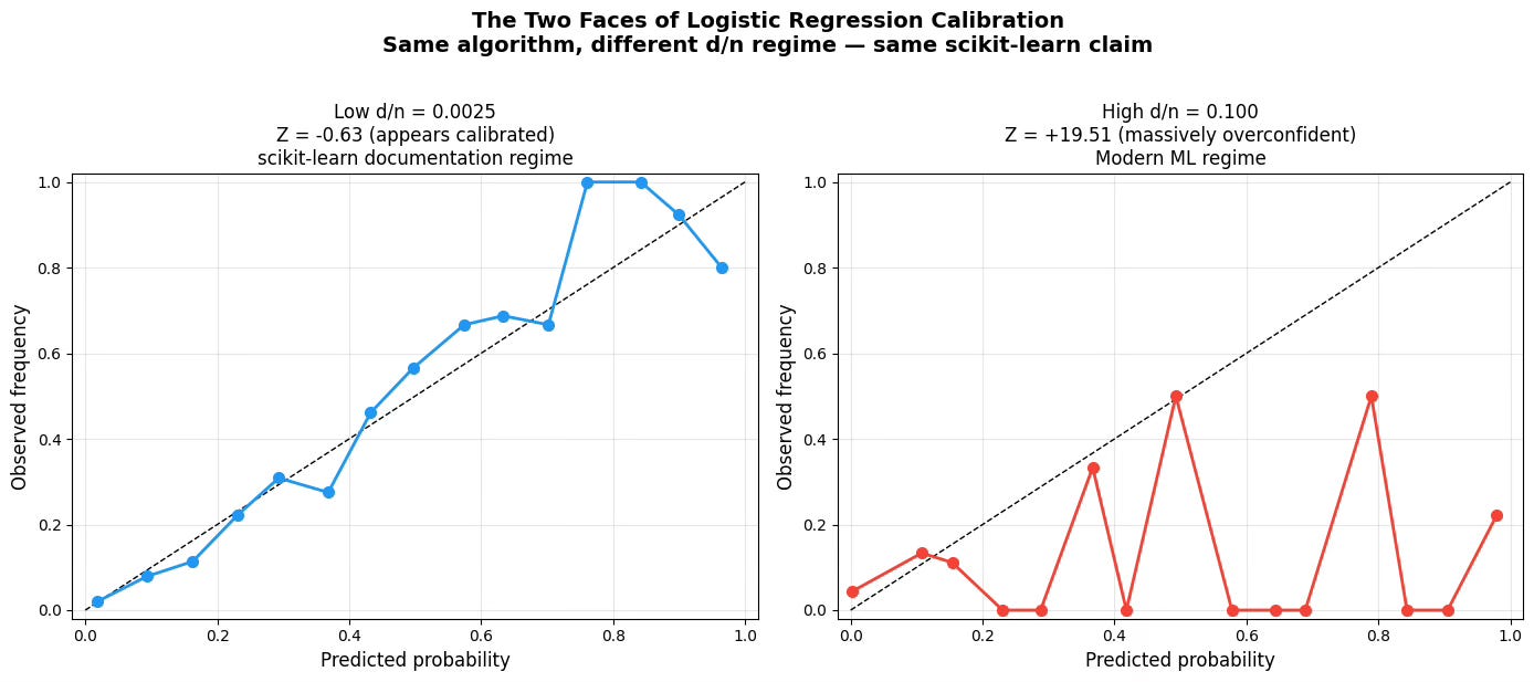
Same model class. Same estimation procedure. Same correctly specified data-generating process. What changed?
The ratio that did it
One number separates the two versions: the ratio of feature dimension to sample size.
Version A has d/n = 50 / 20,000 = 0.0025. Version B has d/n = 200 / 2,000 = 0.10.
That’s it. That is the entire difference. And it is not a quirk of these two particular settings — sweep d/n from small to large and both the Z statistic and the Brier score deteriorate along the way:
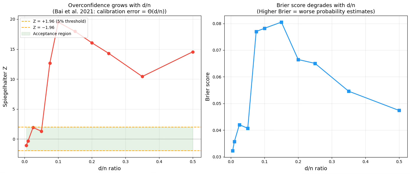
Miscalibration here is not a defect you discover after deployment. It is a property you can read off the shape of your training set before you fit anything.
Why this happens
The classical theory everyone learned — maximum likelihood is asymptotically unbiased, the probabilities converge to the truth — is a statement about d fixed and n going to infinity. In that world, d/n goes to zero and logistic regression is eventually calibrated.
But real problems don’t live in that world. They live at some fixed d/n, and modern high-dimensional theory (Sur and Candès, 2019) shows that when d/n is bounded away from zero, the logistic MLE is systematically biased: the fitted coefficients are inflated in magnitude, and the predicted probabilities are pushed toward 0 and 1. The model becomes overconfident by construction — not because it is wrong about the signal, but because maximum likelihood itself overshoots in this regime.
Two things are worth letting sink in:
Overconfidence is the default failure mode. The bias inflates coefficients, so probabilities near the extremes are too extreme. This is the same direction of failure you see in deep networks — and it emerges in humble logistic regression, with nothing “deep” anywhere in sight.
Ranking survives; numbers don’t. The inflated coefficients still point in the right directions, so the model ranks cases sensibly and discrimination metrics can look fine. Everything I wrote in The fallacy of predict_proba applies: the outputs are monotone scores in [0, 1], not probabilities you can act on.
What to do with this on Monday morning
Compute d/n for the models you have in production. Not as a precise diagnostic — as triage.
If d/n is tiny — thousands of samples per feature — classical intuition roughly holds and calibration failures, if any, come from elsewhere (misspecification, shift).
If d/n is not tiny — and with wide feature sets, one-hot encodings, and modest datasets it usually isn’t — assume miscalibration until a held-out calibration test says otherwise. Run the Spiegelhalter Z on a held-out set. It is a few lines of code and it would have flagged Version B instantly.
The uncomfortable takeaway: “my model is well-specified” is not a calibration defense. Version B was well-specified. Calibration is a property of the estimation regime, not just the model family.
The fix
So the diagnosis is cheap. What about the cure? You cannot just collect ten times more data by Thursday, and you usually cannot throw away three-quarters of your features.
There is a post-hoc fix — one that comes with a mathematical validity guarantee rather than a hope — and on this exact experiment it takes the Brier score from 0.078 to 0.050 and brings the Z statistic back inside the no-rejection band. That is Thursday’s post, for paid subscribers.
This experiment is part of the calibration chapter of Applied Conformal Prediction — the full treatment covers when calibration breaks, how to test it properly, and the calibrators that actually come with guarantees.